4.Iris与集成学习

摘要
第四次机器学习课程实验
仅供参考

---

1. 将数据集按7：3 的比例随机划分为训练集和验证集，随机数生成器种子为学号后三位数431，并输出训练集和验证集前10行数据；

from sklearn.datasets import load_iris
from sklearn.model_selection import train_test_split
import pandas as pd

# 加载数据集
data = load_iris()
X = data.data
y = data.target

# 划分训练集和验证集（7:3比例）
X_train, X_val, y_train, y_val = train_test_split(
    X, y, test_size=0.3, random_state=431
)

# 组合特征和标签，并添加列名
columns = data.feature_names + ['target']
train_data = pd.DataFrame(X_train, columns=data.feature_names)
train_data['target'] = y_train
val_data = pd.DataFrame(X_val, columns=data.feature_names)
val_data['target'] = y_val

# 输出结果
print("训练集前10行数据：")
print(train_data.head(10))
print("\n验证集前10行数据：")
print(val_data.head(10))

<font size=1>训练集前10行数据：
   sepal length (cm)  sepal width (cm)  petal length (cm)  petal width (cm)  \
0                4.7               3.2                1.6               0.2   
1                6.5               3.0                5.5               1.8   
2                4.9               3.1                1.5               0.1   
3                5.6               3.0                4.5               1.5   
4                5.0               3.4                1.5               0.2   
5                5.8               2.6                4.0               1.2   
6                4.9               2.4                3.3               1.0   
7                4.6               3.2                1.4               0.2   
8                5.7               2.6                3.5               1.0   
9                5.4               3.9                1.3               0.4   

   target  
0       0  
1       2  
2       0  
3       1  
4       0  
5       1  
6       1  
7       0  
8       1  
9       0  

验证集前10行数据：
   sepal length (cm)  sepal width (cm)  petal length (cm)  petal width (cm)  \
0                5.4               3.7                1.5               0.2   
1                6.7               3.3                5.7               2.5   
2                5.0               2.0                3.5               1.0   
3                5.1               3.5                1.4               0.3   
4                4.4               3.0                1.3               0.2   
5                4.7               3.2                1.3               0.2   
6                6.4               2.9                4.3               1.3   
7                4.4               3.2                1.3               0.2   
8                5.7               3.0                4.2               1.2   
9                5.1               3.3                1.7               0.5   

   target  
0       0  
1       2  
2       1  
3       0  
4       0  
5       0  
6       1  
7       0  
8       1  
9       0  

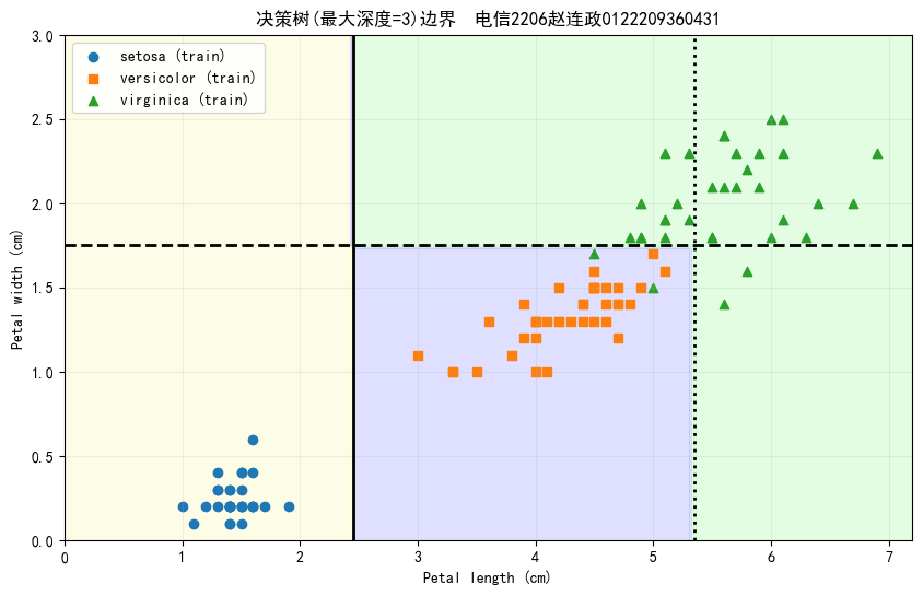
2. 在训练集上训练决策树模型，生成如下的决策树边界

from sklearn.tree import DecisionTreeClassifier
import numpy as np
import matplotlib.pyplot as plt
from matplotlib.colors import ListedColormap
# 设置字体为支持中文的字体
plt.rcParams['font.sans-serif'] = ['SimHei']  # 指定中文字体为黑体
plt.rcParams['axes.unicode_minus'] = False  # 解决负号显示问题
# 选择用于绘制的特征：花瓣长度（第3列）和花瓣宽度（第4列）
X_train_petal = X_train[:, [2, 3]]
X_val_petal = X_val[:, [2, 3]]

# 训练决策树模型（使用花瓣特征）
max_depth = 3
tree_clf = DecisionTreeClassifier(max_depth=max_depth, random_state=431)
tree_clf.fit(X_train_petal, y_train)

# 生成网格数据
x_min, x_max = 0, 7.2
y_min, y_max = 0, 3
xx, yy = np.meshgrid(np.linspace(x_min, x_max, 100),
                     np.linspace(y_min, y_max, 100))

# 预测整个网格的类别
Z = tree_clf.predict(np.c_[xx.ravel(), yy.ravel()])
Z = Z.reshape(xx.shape)

# 创建颜色映射
custom_cmap = ListedColormap(['#fafab0', '#9898ff', '#a0faa0'])

# 绘制决策边界
plt.figure(figsize=(10, 6))
plt.contourf(xx, yy, Z, alpha=0.3, cmap=custom_cmap)

# 绘制训练数据点
markers = ('o', 's', '^')
for idx, marker in zip(range(3), markers):
    plt.scatter(X_train_petal[y_train == idx, 0],
                X_train_petal[y_train == idx, 1],
                marker=marker,
                label=f"{data.target_names[idx]} (train)")

# 提取决策树阈值
def get_thresholds(tree):
    thresholds = []
    features = []
    stack = [0]  # 从根节点开始
    while stack:
        node_id = stack.pop()
        if tree.children_left[node_id] != tree.children_right[node_id]:
            thresholds.append(tree.threshold[node_id])
            features.append(tree.feature[node_id])
            stack.append(tree.children_left[node_id])
            stack.append(tree.children_right[node_id])
    return thresholds, features

thresholds, features = get_thresholds(tree_clf.tree_)

# 绘制决策边界线
line_styles = ['-', '--', ':']
for i, (th, feat) in enumerate(zip(thresholds, features)):
    if feat == 0:  # 花瓣长度
        plt.plot([th, th], [y_min, y_max], 
                 linestyle=line_styles[i%3], 
                 color='k', 
                 linewidth=2)
    elif feat == 1:  # 花瓣宽度
        plt.plot([x_min, x_max], [th, th], 
                 linestyle=line_styles[i%3], 
                 color='k', 
                 linewidth=2)

# 添加标注和美化
plt.title(f"决策树(最大深度={max_depth})边界  电信2206赵连政0122209360431")
plt.xlabel("Petal length (cm)")
plt.ylabel("Petal width (cm)")
plt.axis([x_min, x_max, y_min, y_max])
plt.legend(loc="upper left")
plt.grid(True, alpha=0.2)
plt.show()

3. 在训练集上训练Bagging（基学习器自选）和随机森林模型，基学习器个数为100，输出决策边界图，并分析结果差异；

from sklearn.ensemble import BaggingClassifier, RandomForestClassifier
import matplotlib.pyplot as plt
import numpy as np
from matplotlib.colors import ListedColormap

# 设置基础参数
n_estimators = 100
max_depth = 3  # 保持与之前决策树相同深度
random_seed = 431

# 初始化模型
bagging_clf = BaggingClassifier(
    DecisionTreeClassifier(max_depth=max_depth),
    n_estimators=n_estimators,
    random_state=random_seed
)

rf_clf = RandomForestClassifier(
    n_estimators=n_estimators,
    max_depth=max_depth,
    random_state=random_seed
)

# 训练模型
bagging_clf.fit(X_train_petal, y_train)
rf_clf.fit(X_train_petal, y_train)

# 创建网格数据
x_min, x_max = 0, 7.2
y_min, y_max = 0, 3
xx, yy = np.meshgrid(np.linspace(x_min, x_max, 100),
                     np.linspace(y_min, y_max, 100))

# 定义可视化函数
def plot_decision_boundary(clf, title, ax):
    # 预测网格
    Z = clf.predict(np.c_[xx.ravel(), yy.ravel()]).reshape(xx.shape)
    
    # 绘制决策边界
    custom_cmap = ListedColormap(['#fafab0', '#9898ff', '#a0faa0'])
    ax.contourf(xx, yy, Z, alpha=0.3, cmap=custom_cmap)
    ax.contour(xx, yy, Z, cmap="YlGn", alpha=0.8 )
    # 绘制训练数据点
    markers = ('o', 's', '^')
    for idx, marker in enumerate(markers):
        ax.scatter(X_train_petal[y_train == idx, 0],
                   X_train_petal[y_train == idx, 1],
                   marker=marker,
                   label=data.target_names[idx])
    
    # 美化设置
    ax.set_title(title)
    ax.set_xlabel("Petal length (cm)")
    ax.set_ylabel("Petal width (cm)")
    ax.axis([x_min, x_max, y_min, y_max])
    ax.legend(loc="upper left")
    ax.grid(True, alpha=0.2)

# 创建对比图
plt.figure(figsize=(18, 6))
plt.suptitle('电信2206赵连政0122209360431', fontsize=16, fontweight='bold', y=1.05)
# Bagging决策边界
ax1 = plt.subplot(1, 2, 1)
plot_decision_boundary(bagging_clf, "Bagging (100 Decision Trees)", ax1)

# 随机森林决策边界
ax2 = plt.subplot(1, 2, 2)
plot_decision_boundary(rf_clf, "随机森林 (100 Trees)", ax2)

plt.tight_layout()
plt.show()

# 验证集准确率对比
print(f"Bagging验证集准确率: {bagging_clf.score(X_val_petal, y_val):.3f}")
print(f"随机森林验证集准确率: {rf_clf.score(X_val_petal, y_val):.3f}")

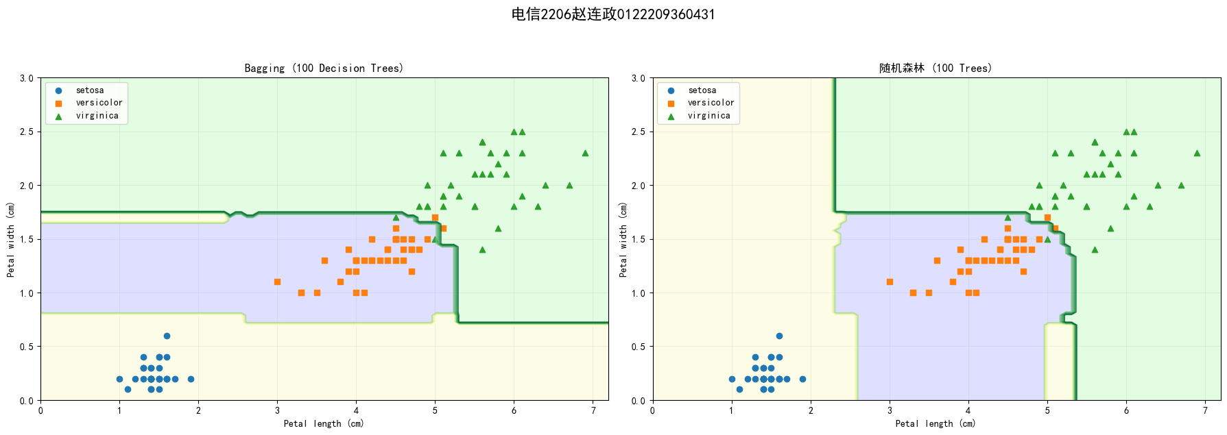
Bagging验证集准确率: 0.978
随机森林验证集准确率: 0.956

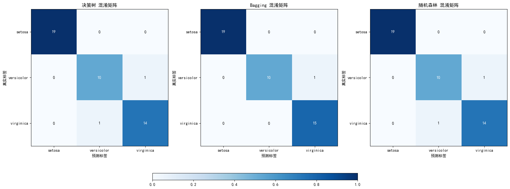
4. 分别计算决策树、Bagging（基学习器自选）和随机森林模型在Iris数据集上三分类的混淆矩阵，并对三种算法的输出结果进行比较.

# 计算混淆矩阵
def print_confusion_matrix(y_true, y_pred, model_name):
    cm = confusion_matrix(y_true, y_pred)
    print(f"{model_name} 混淆矩阵:")
    print(cm)
    print(f"{model_name} 分类报告:")
    print(classification_report(y_true, y_pred))
    return cm

# 绘制混淆矩阵
def plot_confusion_matrix(cm, model_name, ax):
    im = ax.imshow(cm, interpolation='nearest', cmap=plt.cm.Blues)
    ax.set_title(f"{model_name} 混淆矩阵")
    tick_marks = np.arange(len(data.target_names))
    ax.set_xticks(tick_marks)
    ax.set_yticks(tick_marks)
    ax.set_xticklabels(data.target_names)
    ax.set_yticklabels(data.target_names)
    ax.set_xlabel('预测标签')
    ax.set_ylabel('真实标签')
    
    # 添加数值标签
    for i in range(len(data.target_names)):
        for j in range(len(data.target_names)):
            ax.text(j, i, cm[i, j], ha='center', va='center', color='white' if cm[i, j] > cm.max() / 2 else 'black')

    return im

# 计算并打印混淆矩阵
cm_tree = print_confusion_matrix(y_val, y_pred_tree, "决策树")
cm_bagging = print_confusion_matrix(y_val, y_pred_bagging, "Bagging")
cm_rf = print_confusion_matrix(y_val, y_pred_rf, "随机森林")

# 绘制混淆矩阵
fig = plt.figure(figsize=(18, 8))
gs = gridspec.GridSpec(1, 3)

ax0 = fig.add_subplot(gs[0, 0])
ax1 = fig.add_subplot(gs[0, 1])
ax2 = fig.add_subplot(gs[0, 2])

plot_confusion_matrix(cm_tree, "决策树", ax0)
plot_confusion_matrix(cm_bagging, "Bagging", ax1)
plot_confusion_matrix(cm_rf, "随机森林", ax2)

# 添加水平颜色条
cax = fig.add_axes([0.3, 0.15, 0.4, 0.03])  # 调整位置和大小
fig.colorbar(plt.cm.ScalarMappable(cmap=plt.cm.Blues), cax=cax, orientation='horizontal')

plt.tight_layout(rect=[0, 0.2, 1, 1])  # 调整布局以避免颜色条重叠
plt.show()

决策树 混淆矩阵:
[[19  0  0]
 [ 0 10  1]
 [ 0  1 14]]
决策树 分类报告:
              precision    recall  f1-score   support

           0       1.00      1.00      1.00        19
           1       0.91      0.91      0.91        11
           2       0.93      0.93      0.93        15

    accuracy                           0.96        45
   macro avg       0.95      0.95      0.95        45
weighted avg       0.96      0.96      0.96        45

Bagging 混淆矩阵:
[[19  0  0]
 [ 0 10  1]
 [ 0  0 15]]
Bagging 分类报告:
              precision    recall  f1-score   support

           0       1.00      1.00      1.00        19
           1       1.00      0.91      0.95        11
           2       0.94      1.00      0.97        15

    accuracy                           0.98        45
   macro avg       0.98      0.97      0.97        45
weighted avg       0.98      0.98      0.98        45

随机森林 混淆矩阵:
[[19  0  0]
 [ 0 10  1]
 [ 0  1 14]]
随机森林 分类报告:
              precision    recall  f1-score   support

           0       1.00      1.00      1.00        19
           1       0.91      0.91      0.91        11
           2       0.93      0.93      0.93        15

    accuracy                           0.96        45
   macro avg       0.95      0.95      0.95        45
weighted avg       0.96      0.96      0.96        45



C:\Users\86182\AppData\Local\Temp\ipykernel_11464\1982013248.py:50: UserWarning: This figure includes Axes that are not compatible with tight_layout, so results might be incorrect.
  plt.tight_layout(rect=[0, 0.2, 1, 1])  # 调整布局以避免颜色条重叠